3.4 Exercises

Exercise 3.1 First, use a computer simulation to check whether the ML estimator \(\hat{\lambda} = \frac{1}{\text{avg}(x)}\) of \(\lambda\) for the exponential distribution is (at least approximately) unbiased. (See the example for the Poisson distribution above.) Second, prove that the ML estimator of \(\lambda\) is biased. Third, check whether the ML estimator \(\hat{\mu} = \frac{1}{\hat{\lambda}}\) of \(\mu = \frac{1}{\lambda}\) is biased.

Explain the implications for the analysis of UK government duration.

Solution

lambda <- 4.0      # the parameter we're trying to estimate
sample_size <- 10  # the sample size we're using in each "study"

n_repeated_samples <- 10000  # the number of times we repeat the "study"
lambda_hat <- numeric(n_repeated_samples)  # a container 
for (i in 1:n_repeated_samples) {
  x <- rexp(sample_size, rate = lambda)
  lambda_hat[i] <- 1/mean(x)
}

# long-run average
mean(lambda_hat)  # hum... seems too big

## [1] 4.436498

\[ \begin{aligned} E\left[ \frac{1}{\text{avg}(x)}\right] = E\left[ \frac{N}{\sum_{n = 1}^N x_n}\right] &= N E \left[ \frac{1}{ \sum_{n = 1}^N x_n} \right] \\ \text{[notice the greater-than sign here]} \rightarrow & > N \left[ \frac{1}{ E \left( \sum_{n = 1}^N x_n \right) } \right] \text{, by Jensen's inquality; } \frac{1}{x} \text{ is convex.}\\\\ & = N \left[ \frac{1}{ \sum_{n = 1}^N E(x_n) } \right] \\ & = N \left[ \frac{1}{ \sum_{n = 1}^N \frac{1}{\lambda} } \right] \\ & = N \left[ \frac{1}{ \frac{N}{\lambda} } \right] \\ & = \lambda \end{aligned} \] Therefore the bias in \(\hat{\lambda}\) is upward, as the simulation shows.

Remember that we can transform ML estimators directly to obtain estimates of the transformations. The ML estimator \(\hat{\mu} = \frac{1}{\hat{\lambda}}\) of the average duration \(\mu = \frac{1}{\lambda} = E(X)\) is unbiased, though. The math works nearly identically as the math showing that the ML estimator for the toothpaste cap problem. It also follows directly from the fact that the sample average is an unbiased estimator of the population average.

Exercise 3.2 The ML estimator \(\hat{\lambda} = \frac{1}{\text{avg}(x)}\) of \(\lambda\) for the exponential distribution is consistent. Comment on the relevance for Exercise 2.6.

Solution

Consistency is not helpful for this problem. We have five observations. At best, consistency suggests an estimator will work well in large samples. A consistent estimator can be heavily biased in small samples.

Exercise 3.3 Comment on the ML estimator \(\hat{\lambda} = \frac{1}{\text{avg}(x)}\) of \(\lambda\) for the exponential distribution and the ML estimator \(\hat{\mu} = \frac{1}{\hat{\lambda}}\) of the \(\mu = \frac{1}{\lambda}\). Comment on the relevance for Exercise 2.6.

Solution

Both estimators are consistent. However, consistency is not helpful in small samples.

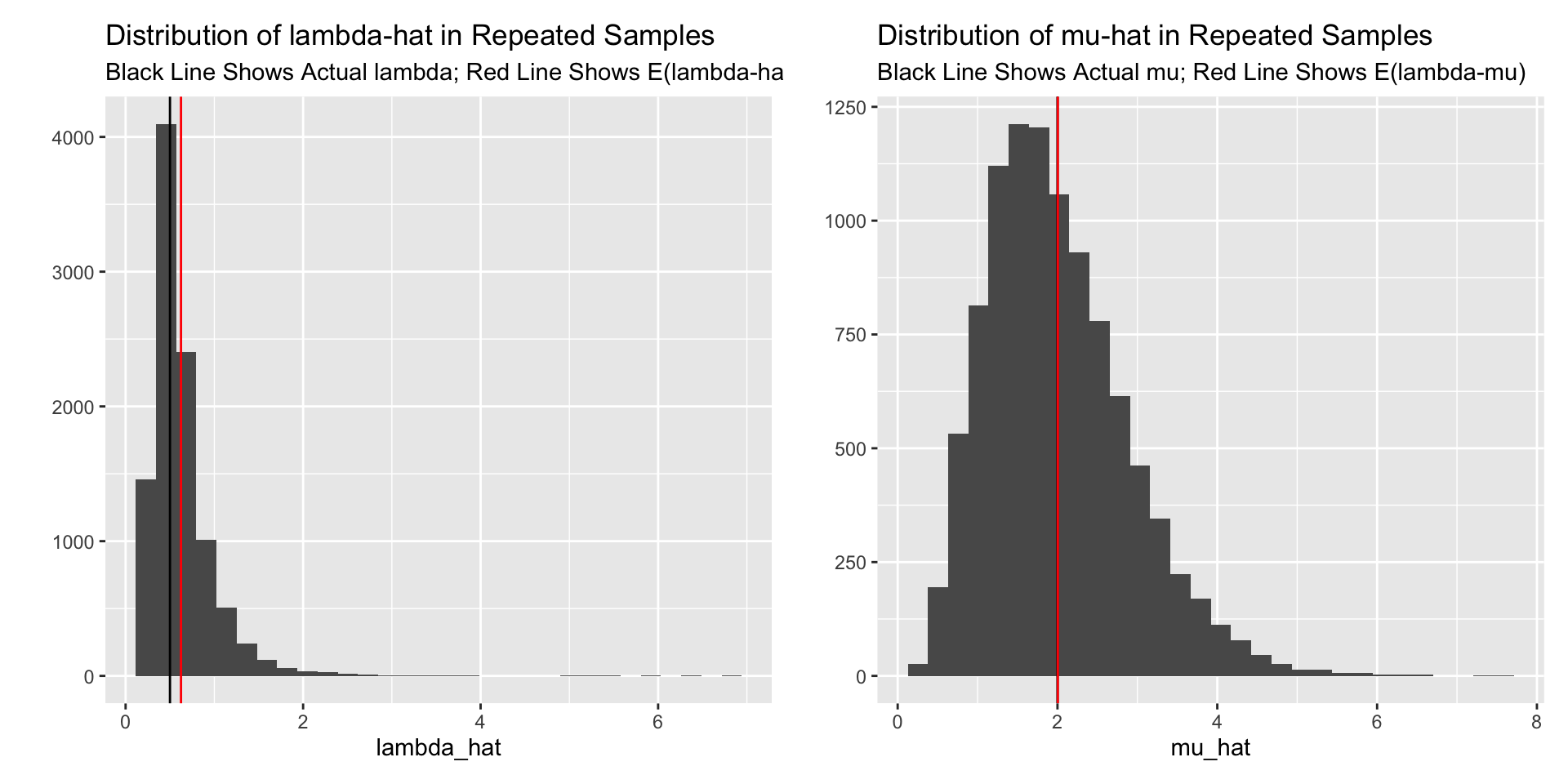
\(\hat{\mu}\) is unbiased, and \(\hat{\lambda}\) is biased. This leads us to prefer \(\hat{\mu}\). Further \(\hat{\mu}\) is the MVUE, because it’s the sample average used to estimate the expected value of the distribution. MVUE is an excellent estimator and it’s unusually to prefer another. \(\hat{\mu}\) has much better properties than \(\hat{\lambda}\)—\(\hat{\mu}\) is an MVUE, \(\hat{\lambda}\) is just consistent.

Perhaps more importantly, \(\hat{\mu}\) is easier to interpret as the expected years a government will last. \(\hat{\lambda}\) is a bit harder to interpret at the failures per year.

Here’s a little simulation illustrating each estimator.

lambda <- 0.5     # a guess at the value in the govt duration problem
sample_size <- 5  # the sample size in the govt duration problem

n_repeated_samples <- 10000  # the number of times we repeat the "study"
lambda_hat <- numeric(n_repeated_samples)  # a container 
mu_hat <- numeric(n_repeated_samples)      # another container 
for (i in 1:n_repeated_samples) {
  x <- rexp(sample_size, rate = lambda)
  lambda_hat[i] <- 1/mean(x)
   mu_hat[i] <- mean(x)
}

# long-run average
mean(lambda_hat)  # hum... seems too big

## [1] 0.6240386

mean(mu_hat)      # just right!

## [1] 2.004443

library(ggplot2)
library(patchwork)
gg1 <- qplot(x = lambda_hat) + 
  geom_vline(xintercept = lambda) + 
  geom_vline(xintercept = mean(lambda_hat), color = "red") + 
  labs(title = "Distribution of lambda-hat in Repeated Samples",
       subtitle = "Black Line Shows Actual lambda; Red Line Shows E(lambda-hat)")
gg2 <- qplot(x = mu_hat) + 
  geom_vline(xintercept = 1/lambda) + 
  geom_vline(xintercept = mean(mu_hat), color = "red") + 
  labs(title = "Distribution of mu-hat in Repeated Samples",
       subtitle = "Black Line Shows Actual mu; Red Line Shows E(lambda-mu)")

gg1 + gg2